introduction
许多Web应用程序的预测任务需要建模分类变量,例如用户ID以及性别和职业等人口统计信息。
Many web applications’ predictive tasks involve modeling categorical variables such as user IDs, demographics like gender and occupation, and more. To apply standard machine learning techniques, these categorical predictive variables are typically converted into a set of binary features through one-hot encoding, resulting in highly sparse feature vectors. To effectively learn from such sparse data, it’s crucial to consider interactions between these features.
为了应用标准的机器学习技术,这些分类预测变量通常会通过独热编码转换为一组二进制特征,使得生成的特征向量高度稀疏。为了有效地从这样的稀疏数据中学习,必须考虑特征之间的相互作用。
Factorization Machines (FMs) are a popular solution for efficiently modeling second-order feature interactions. However, FM models handle feature interactions in a linear manner, which may not capture the nonlinearity and complex underlying structures in real-world data. While deep neural networks have been applied recently to learn non-linear feature interactions in industry, such as Google’s Wide & Deep and Microsoft’s DeepCross, deep structures make them challenging to train.
因子分解机(FMs)是用于高效使用二阶特征交互的流行解决方案。
但是,FM模型以线性方式处理特征交互,这可能无法捕捉现实世界数据的非线性和复杂内在结构。虽然深度神经网络最近已被应用于学习行业中的非线性特征交互,例如Google的Wide&Deep和微软的DeepCross,但深层结构同时使它们难以训练。
在本文中,我们提出了一种新颖的模型——神经因子分解机(NFM),用于处理稀疏环境下的预测。
In this paper, we introduce a novel model called Neural Factorization Machine (NFM) for handling predictions in sparse environments. NFM seamlessly combines the linear properties of FMs in modeling second-order feature interactions and the non-linear properties of neural networks in modeling high-order feature interactions.
NFM无缝地结合了FM在建模二阶特征交互方面的线性性质和神经网络在建模高阶特征交互方面的非线性性质。
从概念上讲,NFM比FM更具表现力,因为FM可以看作是没有隐藏层的NFM的特殊情况。在两个回归任务的实证结果中,仅使用一个隐藏层的NFM相对于FM显著提高了7.3%。
In concept, NFM is more expressive than FM, as FM can be seen as a special case of NFM without hidden layers. In empirical results on two regression tasks, a single hidden layer NFM significantly outperforms FM by 7.3%.
与最近的深度学习方法Wide&Deep和DeepCross相比,我们的NFM结构更浅,但性能更好,实际中更容易训练和调整。
Compared to recent deep learning approaches like Wide & Deep and DeepCross, our NFM structure is shallower but performs better and is easier to train and tune in practice.
痛点
NFM (Neural Factorization Machine) can be seen as an improvement over both FM (Factorization Machines) and FNN (Deep Factorization Neural Network), addressing their respective shortcomings as follows:
NFM(神经因子分解机)可以被视为对FM(因子分解机)和FNN(深度因子分解神经网络)的改进,分别解决了它们的缺点如下:
FM Model Limitation: While the FM model effectively captures cross-feature interactions, it still models these interactions linearly, which means it cannot capture non-linear relationships between features.
FM 模型的限制: 虽然FM模型有效地捕捉了特征之间的交叉相互作用,但它仍然线性地建模这些相互作用,这意味着它不能捕捉特征之间的非线性关系。
FNN Model Limitation: The FNN model attempts to overcome the limitations of FM by using FM for feature vector initialization at the lower layers and then using a DNN (Deep Neural Network) to learn high-order non-linear features at the upper layers. However, it relies on concatenating individual feature embeddings and then learning cross-feature interactions in subsequent DNN layers. In practical applications, this approach may not effectively capture cross-feature interactions to the desired extent.
FNN 模型的限制: FNN模型试图通过在较低层使用FM进行特征向量初始化,然后在较高层使用DNN(深度神经网络)来学习高阶非线性特征来克服FM的限制。然而,它依赖于连接各个特征嵌入,然后在随后的DNN层中学习跨特征的相互作用。在实际应用中,这种方法可能无法有效捕捉跨特征的相互作用到所需的程度。
Therefore, there was a need for a model that could both learn high-order features and capture non-linear relationships effectively, which led to the development of the NFM model.
因此,有必要开发一种既能够学习高阶特征又能够有效捕捉非线性关系的模型,这就引出了NFM模型的发展。
目标函数
The objective function of the NFM (Neural Factorization Machine) model is typically represented as follows:
NFM(神经因子分解机)模型的目标函数通常表示如下:
[ \text{NFM Loss} = -\frac{1}{N} \sum_{i=1}^{N} \left( y_i \log(\hat{y}_i) + (1 - y_i) \log(1 - \hat{y}_i) \right) + \lambda \cdot \Omega(\theta) ]
Where:
- (N) is the number of training examples.
- (y_i) represents the true label for the (i)-th example.
- (\hat{y}_i) is the predicted output (probability) for the (i)-th example by the NFM model.
- (\lambda) is the regularization parameter.
- (\theta) represents the model’s parameters.
- (\Omega(\theta)) is the regularization term used to prevent overfitting. It can be L1 regularization, L2 regularization, or a combination of both.
其中:
- (N) 是训练示例的数量。
- (y_i) 表示第 (i) 个示例的真实标签。
- (\hat{y}_i) 是NFM模型对第 (i) 个示例的预测输出(概率)。
- (\lambda) 是正则化参数。
- (\theta) 代表模型的参数。
- (\Omega(\theta)) 是用于防止过拟合的正则化项。它可以是L1正则化、L2正则化或二者的组合。
The goal of training the NFM model is to minimize this loss function, which combines a logistic loss term to measure the prediction error and a regularization term to control the complexity of the model. By minimizing this objective function, the model aims to make accurate predictions while avoiding overfitting.
训练NFM模型的目标是最小化这个损失函数,它结合了用于度量预测误差的逻辑损失项和用于控制模型复杂性的正则化项。通过最小化这个目标函数,模型旨在进行准确的预测,同时避免过拟合。
network 结构
I apologize for the previous response, but I’m unable to view or interpret images or diagrams. However, I can describe the typical architecture of an NFM (Neural Factorization Machine) model in text.
NFM(神经因子分解机)模型的典型架构如下,它将因子分解机(Factorization Machines,FMs)和神经网络的优势结合起来,以捕获特征之间的线性和非线性交互:
The NFM architecture combines the strengths of Factorization Machines (FMs) and neural networks to capture both linear and non-linear interactions between features. Here’s a textual representation of the NFM structure:
Input Layer: The model takes input features, which are usually one-hot encoded or embedded into continuous vectors.
输入层: 模型接受输入特征,通常这些特征是进行独热编码或嵌入成连续向量的形式。
Embedding Layer: Each input feature is passed through an embedding layer, which converts them into dense vectors. These dense vectors capture the latent representations of the features.
嵌入层: 每个输入特征通过嵌入层,被转换为密集向量。这些密集向量捕获了特征的潜在表示。
Pairwise Interaction Layer (Factorization Machine): The pairwise interaction layer calculates the interactions between all pairs of feature embeddings. It computes the dot product between each pair of embeddings and then aggregates these interactions. This step captures second-order feature interactions and is similar to the FM component.
二阶交互层(因子分解机): 二阶交互层计算特征嵌入之间的所有特征对的交互。它计算每一对嵌入之间的点积,然后汇总这些交互作用。这一步捕获了二阶特征交互,类似于FM组件。
Fully Connected Neural Network: In addition to the FM component, the NFM includes a fully connected neural network or deep learning layers. These layers can have multiple hidden layers and neurons, allowing the model to learn complex, high-order feature interactions. This part of the network captures non-linear relationships among features.
全连接神经网络: 除了FM组件,NFM还包括一个完全连接的神经网络或深度学习层。这些层可以有多个隐藏层和神经元,使模型能够学习特征之间的复杂高阶交互。这部分网络捕获了特征之间的非线性关系。
Output Layer: The final layer typically consists of a single neuron with a sigmoid activation function. It produces the predicted output, which represents the probability of the positive class in a binary classification problem.
输出层: 最后一层通常由一个具有Sigmoid激活函数的单个神经元组成。它产生了预测输出,表示在二元分类问题中正类别的概率。
Objective Function: The model is trained to minimize an objective function, usually a combination of a logistic loss term (to measure prediction error) and a regularization term (to prevent overfitting).
目标函数: 模型的训练目标是最小化一个目标函数,通常是逻辑损失项(用于度量预测误差)和正则化项(用于防止过拟合)的组合。
The NFM architecture leverages both the FM component for capturing pairwise feature interactions and the neural network component for modeling higher-order, non-linear interactions. This combination makes it capable of learning complex patterns in the data.
NFM架构充分利用了FM组件来捕获特征的成对交互,同时还使用神经网络组件来建模高阶、非线性交互。这种组合使其能够学习数据中的复杂模式。


